Sizing an air conditioner (or heat pump) shouldn’t be left to guesswork. That’s why we have engineering protocols like ACCA Manual J for calculating the amount of cooling load a house experiences. Among the factors that contribute are the outdoor and indoor temperatures. But how much cooling load variation do you get if you use inputs other than the design temperatures? Let’s look at an example.

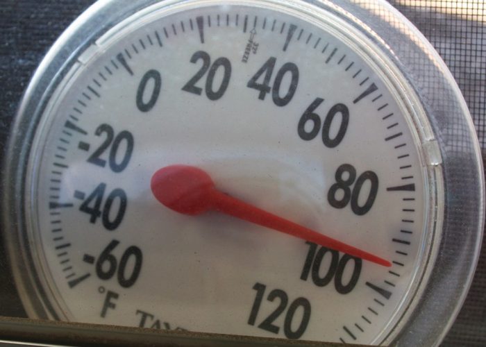
Outdoor temperature

I’ve written quite a bit about the house I bought in 2019. In a recent article, I wrote about how well my Mitsubishi heat pump performed in the arctic blast last December. Before that I wrote about how well it did in last summer’s heat wave. Today, I’ve got some modeling data for you about cooling load variation for my house using the load calculation I did when I did the HVAC design in 2019.

First, let’s look at how the total cooling load (sensible plus latent) changes when I change the outdoor dry bulb temperature. The graph below shows the results. The starred point is the reference for all the other data shown. That’s the design cooling load based on the 1 percent outdoor design temperature of 93°F. The horizontal axis shows excursions from the design temperature in degrees Fahrenheit. The vertical axis shows the percent change in the cooling load as the outdoor temperature varies.

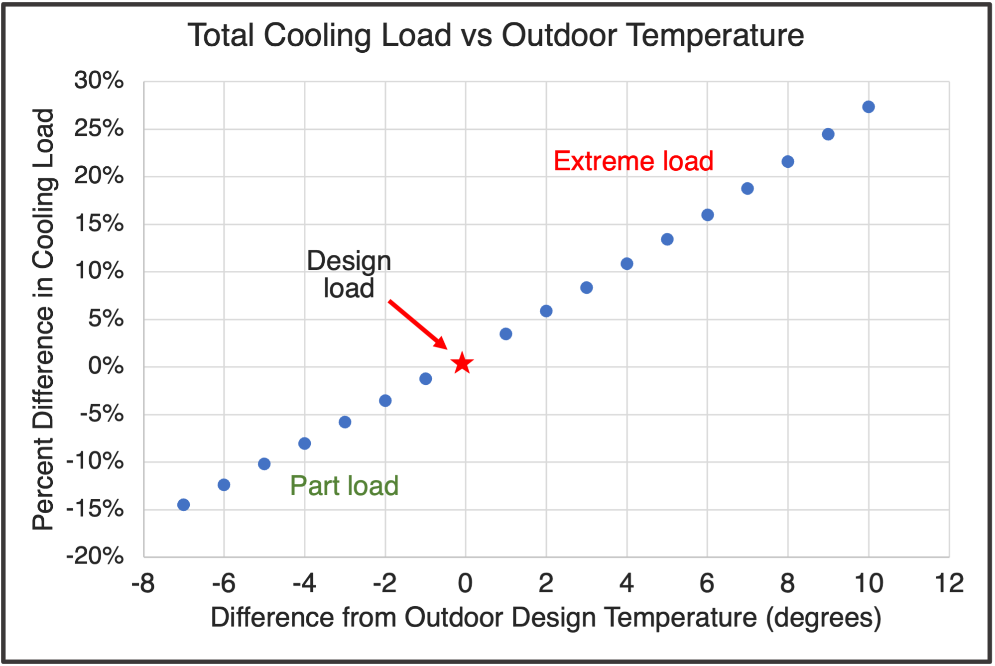
With outdoor temperatures lower than the design temperature, the cooling load decreases. Those are considered part-load conditions. As the outdoor temperature goes above the design temperature, the cooling load increases. That’s the extreme load side.

As you can see, the cooling load increases significantly with higher outdoor design temperature. An increase of just 2°F results in 6% more total cooling load. Going up 5°F, from 93 to 98°F, increases the load 13%. And with a 10°F increase, the total cooling load grows by 27%. In my house, that 10°F increase means the cooling load goes from 21 kBTU/hr to 27 kBTU/hr.

In short, changing the outdoor temperature increases or decreases the cooling load by ~2.7% for each degree of increase or decrease in this example.

What about outdoor humidity?

In the analysis above, I’ve changed only the outdoor dry bulb temperature. The HVAC design software we use at Energy Vanguard is RightSuite Universal, and it deals with the humidity (latent load) in an interesting way. It keeps the outdoor wet bulb temperature constant. What that means is that the latent load, the part related to removing humidity, actually goes down as the outdoor dry bulb temperature goes up.

It’s certainly possible that the latent load will go up as the outdoor temperature increases, but let’s focus just on the part related to changing dry bulb temperature, the sensible load. The graph below pulls out just the sensible load.

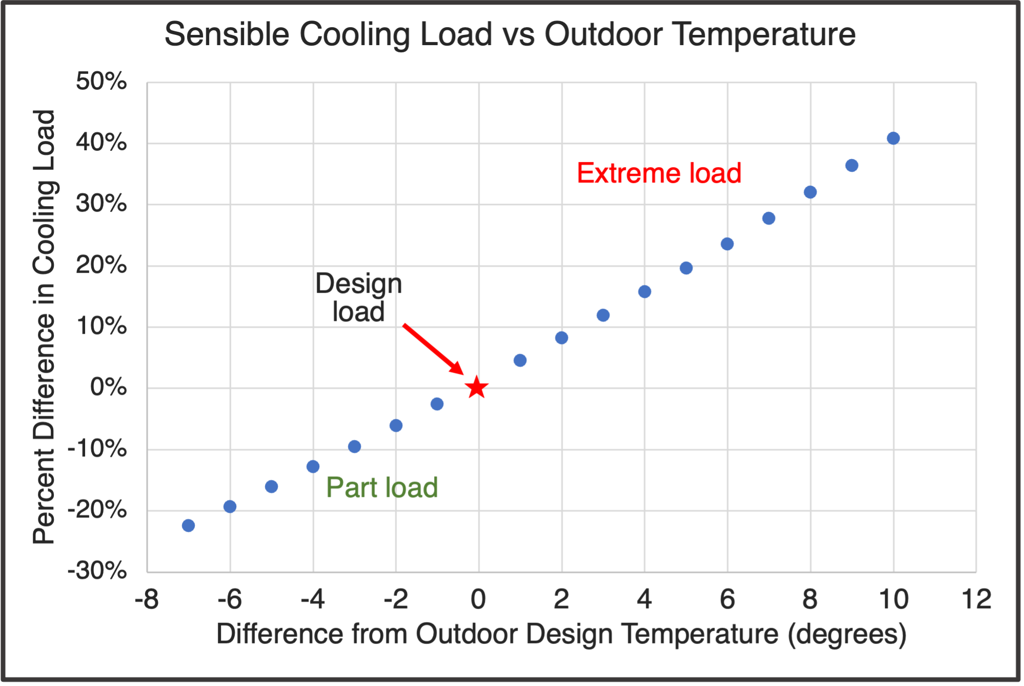
Everything is the same here except for the scale. Now, a 5°F increase from 93 to 98°F increases the load 20%. A 10°F increase blows up the total cooling load by 41% In my house, that means the sensible load goes from 17.5 kBTU/hr to 24.7 kBTU/hr.

Indoor temperature

OK, what happens if you leave the outdoor temperature at the 1% design temperature but change the indoor temperature. That’s your thermostat set point. Again, we’re changing only the dry bulb temperature. The software this time deals with the humidity by keeping the indoor relative humidity constant at 50%.

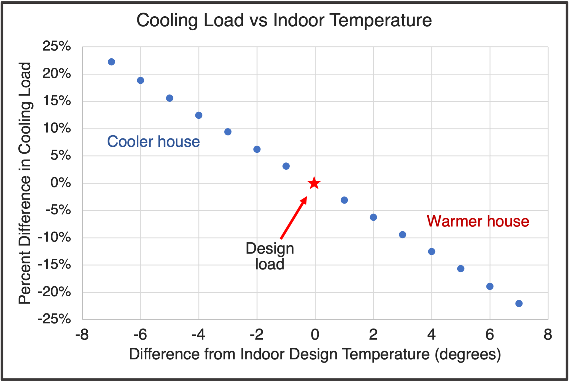
The graph above is similar to the other two. The slope of the curve is different because increasing the thermostat set point keeps the house warmer, which means less air conditioning. The percent change in cooling load is similar to what happens to the total cooling load when you change the outdoor temperature.

The Manual J indoor design temperature is 75°F. A 2°F decrease, from 75 to 73°F, results in 6% more total cooling load. Keeping the thermostat at 70°F, a 5 degree drop, adds nearly 16% more load. And keeping the thermostat at 68°F increases the cooling load by 22%.

On the humidity side, by keeping the relative humidity constant at 50%, the latent load increases as you lower the indoor temperature. That causes the change in sensible load to be less than the change in total load in this case.

In short, changing the indoor temperature increases or decreases the cooling load by ~3% for each degree of decrease or increase in this example.

Takeaways

If your goal is to cheat on a Manual J load calculation, the above graphs make clear that changing the outdoor and indoor set points can help you do that. But that’s also one of the easiest things for someone checking the reports to find. But my point here is simply to show the cooling load variation you get as the outdoor or indoor temperatures change.

For those of you who do heating and cooling load calculations and HVAC design, changing the design temperatures is a form of bracketing. You find the range of cooling loads that might be reasonable. If, for example, you’re looking at selecting a piece of cooling equipment that’s right on the edge, going through an exercise like this can confirm your choice or perhaps lead you to select different equipment.

Keep in mind that the Manual J load calculation protocol does result in heating and cooling loads that are higher than the actual loads. There’s buffer built into it, so you’ll get a load that’s 10 to 30 percent higher than actual just using the standard inputs. Also, be aware that the equipment selection protocol, Manual S, allows you to size a cooling system at 90 percent of the Manual J load.

Of course, outdoor and indoor design temperatures are only one of the many variables that can affect your heating and cooling loads. Another biggie is infiltration rate. How far off might your load calculation be if you don’t have a blower-door test result and make a bad guess? Hmmmm.

________________________________________________________________________

Allison A. Bailes III, PhD is a speaker, writer, building science consultant, and the founder of Energy Vanguard in Decatur, Georgia. He has a doctorate in physics and is the author of a bestselling book on building science. He also writes the Energy Vanguard Blog. For more updates, you can subscribe to the Energy Vanguard newsletter and follow him on LinkedIn. Images courtesy of author.